EMI and radio links
Two domains that work together. EMI (lagrange_emi, every 1 ms) computes the disturbance
fields of sources in the scene, a power line, a motor drive, a welder, a transmitter, at each
victim, and what they do to it. Comms (lagrange_comms, every 10 ms) computes the quality of
each radio link and CAN bus, with that interference in its noise. The sensors, the ros2_control
bridge and the ROS 2 bridge then apply the results: a magnetometer heading that swings near a
power line, encoder glitches, lost and late messages.
This is behaviourally correct interference for testing robot software. It is not an electromagnetic compatibility certification tool.
flowchart LR
    SRC["EmiSourceAPI_1<br/>power line, motor drive,<br/>welder, transmitter"] --> EMI["EMI<br/>1 ms"]
    MC["motor/*/current_q"] --> EMI
    EMI -->|"b_field"| MAG["Magnetometer"]
    EMI -->|"accel_noise, gyro_noise"| IMU["IMU"]
    EMI -->|"glitch_probability"| ENC["Encoders<br/>(ros2_control)"]
    EMI -->|"bit_error_rate"| CAN["CAN bus"]
    EMI -->|"interference_power"| LINK["Radio link"]
    CAN --> COMMS["Comms<br/>10 ms"]
    LINK --> COMMS
    COMMS -->|"packet loss, latency"| ROS["ROS 2 bridge<br/>--link-topics"]
The EMI equations
Sources. Each is analytic, or a NanoVDB field map in the source’s frame scaled by its
current. Alternating sources carry \(\sqrt2\,(\sin\omega t + \sum_k h_k \sin k\omega t)\) at the
scene’s emi:frequency, which is a site parameter with no default (50 or 60 Hz by region).
A power line is an infinite straight conductor, by the right-hand rule: $\(B = \frac{\mu_0 I}{2\pi d}, \qquad \mu_0 = 1.25663706212\times10^{-6}\ \mathrm{N\,A^{-2}}\)$
A motor drive and a welder are magnetic dipoles along
emi:direction, of momentemi:dipoleMomentPerAmperetimes the current (the motor’scurrent_qwhen the electrical network runs); the welder’s duty cycle is an RMS weight: $\(\mathbf B = \frac{\mu_0}{4\pi}\,\frac{3\,\hat r(\hat r\cdot\mathbf m) - \mathbf m}{r^3}\)$A transmitter is a free-space far field, RMS: $\(E = \frac{\sqrt{30\,P_{EIRP}}}{d}\)$
A wire (RFC 0013) is the sum over the straight segments of its route
emi:path, each by Biot–Savart (Griffiths, Introduction to Electrodynamics, Example 5.5), the return conductoremi:returnOffsetaway carrying the current back: $\(B = \frac{\mu_0 I}{4\pi d}\,(\sin\theta_2 - \sin\theta_1)\)$ Its current is any signal (emi:currentSignal, e.g. a motor’sbus_current), its sign kept. Direct sources add as vectors (a lead and its return cancel), alternating ones in power.
Distances under 1 cm are taken as 1 cm.
Victims (EmiSusceptibilityAPI_1; emi.coupling in the profile picks which are active):
Victim |
Effect |
|---|---|
Magnetometer |
adds the instantaneous \(\mathbf B\), scaled by |
IMU |
Gaussian noise of RMS proportional to \(\lvert E\rvert\) on the accelerometer and gyro |
Encoder |
each edge an extra or missing count with probability \(p = 1/\big(1 + (E_{50}/\lvert E\rvert)^4\big)\) |
CAN bus |
bit-error rate \(\mathrm{BER} = \mathrm{BER}_0\,(\lvert E\rvert/E_{ref})^2\), capped at 0.5 |
Radio |
interference power \(P = \frac{E^2}{Z_0}\,\frac{\lambda^2}{4\pi}\) times the band overlap |
Harness loop |
induced voltage \(V = 2\pi f B A_{loop}\) (RMS) |
The encoder and CAN curves are behavioural, chosen to give a threshold you can set; they are not
derived from first principles. The parameters exist so that someone with measurements can fit
them. A per-victim emi:shieldingEffectiveness stands for shielding.
A robot’s own wiring
The current a robot’s motors draw runs through its battery leads, and that field is what
disturbs its compass most: ArduPilot’s and PX4’s compass calibrations (“compassmot”) fit it as a
field proportional to the current, and aeromagnetic surveys of multicopters measure it so
(Tuck et al., Geosci. Instrum. Method. Data Syst. 10, 2021: 2.8 nT/A for a quadrotor’s
airframe 10 cm below a sensor, linear in the current). --emi-motor-leads SPACING[,X,Y,Z] lays a
wire from the battery (at X,Y,Z on the root link) to each motor, carrying its
motor/<m>/bus_current, its return SPACING m above it, and makes every magnetometer a victim:
lagrange_server --robot assets/robots/quad_x500/quad_x500.usda --world none --air-density 1.225 \
  --geo-origin 47.397742,8.545594,488 --emi-motor-leads 0.005,-0.06,0,-0.06
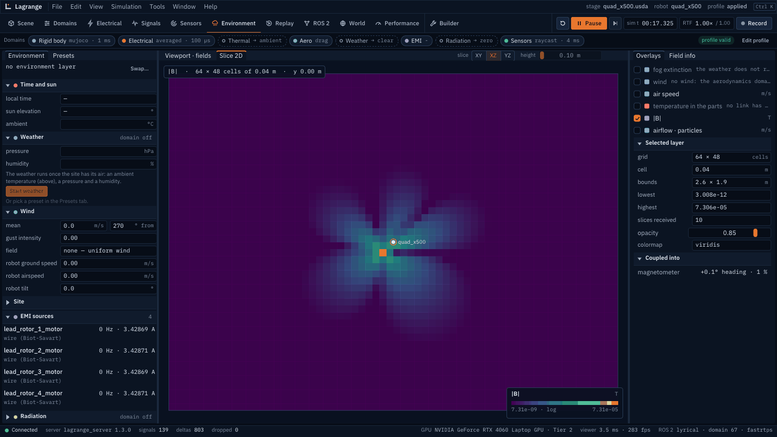
Each such magnetometer also writes sensor/<n>/heading_error (rad, the heading from the
disturbed horizontal field less the heading from the Earth’s) and sensor/<n>/interference
(|disturbance| / |Earth’s field|, what ArduPilot reports as a percentage: under 30 % fine, over
60 % move the compass). The viewer’s Environment workspace slices |B| through the robot (XZ, YZ;
4 cm cells when every source rides on it; a log colour scale) and lists the effects under
Coupled into: each compass’s heading error and share, coloured by those bands, each CAN
bus’s bit-error rate, each radio link’s SNR and loss. A straight lead from the battery to a
motor is the simplest route; a real harness is authored as wire prims with its own path. The
switching noise of the drives on GNSS and radios is not modelled (measured on UAS: C/N0 down by
up to 10 dB with everything on, Stubbs and Akos, GPS World, 2016; an industrial drone’s
electronics cut a GPS module’s sensitivity by 10 dB, 6 dB in simulation, IEICE technical report,
2024-08, https://ken.ieice.org/ken/paper/20240806kcEx/eng/, TODO(verify) the geometry and
source). No published measurement isolates the motor drives, so there is nothing to fit yet.
The radio equations
Received power. Log-distance path loss from Friis at a reference distance \(d_0\), plus a fixed
loss for each wall the straight line from transmitter to receiver crosses (the fixed scenery’s
collision shapes, comms:wallLoss each), plus log-normal shadowing correlated over the
receiver’s travel (Gudmundson):
Noise and SNR. Thermal noise times the noise figure, plus the EMI domain’s interference:
Packets. Bit errors in additive white Gaussian noise for BPSK and QPSK (exact) and 16- and
64-QAM (nearest-neighbour approximation), one symbol per hertz; for BPSK
\(p_b = Q\big(\sqrt{2\,E_b/N_0}\big)\). packet_error_rate is the loss after comms:maxRetries,
latency the expected airtime with retries, throughput the bit rate times the delivered
fraction, and the link is up while at least half the packets arrive.
CAN fault confinement (ISO 11898-1): the frame error rate follows from the bit-error rate; the transmit error counter rises by 8 on an error and falls by 1 on a success, the node is error passive above 127 and bus off above 255, and recovers after 128 × 11 recessive bits. The bus is taken as fully loaded by the node, the worst case.
Applied. lagrange_server --link-topics FILE.yaml puts ROS 2 topics on a link: each message
is lost with the link’s packet loss (always while it is down) and the rest arrive its latency
later, with their original stamps; incoming /cmd_vel too.
Computing it
Both run on the CPU on every tier: a few analytic evaluations per victim, and a handful of ray casts per link for the walls (Embree). Powers and ratios on the bus are linear SI values; decibels appear only in the viewer.
How far to trust it
Check |
Result |
Test |
|---|---|---|
Field of a straight conductor and of a dipole |
closed form within 1e-6 relative |
|
Transmitter far field |
Friis within 1e-6 relative |
|
Mains aliasing |
a 60 Hz field sampled at 100 Hz peaks at 40 Hz, exactly |
|
The sample: 400 A line, quadcopter 9.9 m away |
8.08 µT RMS, as \(\mu_0 I/(2\pi d)\) gives |
a run of |
Behavioural victim curves, shielding, harness pickup |
as specified |
|
Free-space path loss and noise floor |
Friis within 1e-9 relative; \(kTB\) exact |
|
Bit-error curves |
the BPSK 1e-5 point and Q(3) |
|
CAN fault confinement |
transitions exact (transmit counter) |
|
Walls and shadowing |
wall count; shadowing spread |
|
Field near a real power line against published measurements |
owed |
— |
Heading error of a real robot near a known source |
owed: no recording (Q16) |
— |
Indoor path-loss parameters traced to ITU-R P.1238 |
owed, TODO(verify) |
— |
RSSI of a real AMR driving away from an access point |
owed: no recording (Q16) |
— |
Not modelled: occlusion and shielding by the scene’s geometry (beyond the per-victim factor), two-ray ground reflection, low-frequency E fields, the welder’s on/off timing; for radio, coding gain, MAC contention, multipath and fast fading; the CAN receive error counter; the MAVLink bridge’s telemetry on a link.
The full models and their signals are in emi.md and comms.md.