Domain: rotor downwash and outwash¶
The air a rotor pushes, and what it does to everything else. The loads on a rotor itself (thrust, torque, blade-element momentum, ground effect) are in aerodynamics.md §2. This document covers the wake that leaves the rotor: the column of air under a drone, the jet it becomes further down, and the outwash along the ground.
1. Scope¶
What |
Where it acts |
Status |
|---|---|---|
Near wake of each rotor (actuator disc) |
other robots’ links and rotors |
done |
Merged jet below a multirotor |
the same |
done |
Outwash along the ground |
the same; dust lifted for the weather |
done |
Wake skew in wind and forward flight |
the column’s direction |
done |
Live view of the air in the viewer |
|
done (§5) |
Inflow above the disc, swirl, unsteadiness |
not modelled |
|
Interference between rotors of one drone |
not modelled |
|
Buildings: roofs, walls beside a wake (boxes of the scenery) |
the same |
done (§2.6) |
A wall beside a rotor: more inflow, less thrust, a roll towards it |
the robot’s own rotors |
done (§2.7) |
Ceilings, scenery other than boxes and the ground plane |
not modelled |
|
Tethers in the wake, the drone’s own included |
each cable’s masses ( |
done (§2.9) |
The model is aerodynamics::Downwash (modules/aerodynamics/include/lagrange/aerodynamics/Downwash.hpp),
run by the aerodynamics domain (AeroDrag). It runs whenever the stage has rotors and the site
air density is known; the profile’s aerodynamics.downwash: false turns it off.
2. The model¶
flowchart TB
R["Rotor: v_i, thrust axis n<br/>(rotor_aero)"] --> N["Near wake per rotor<br/>actuator disc, s < 1.5 l"]
N --> B{"Merging<br/>1.5 l to 2.5 l"}
B --> F["Merged jet<br/>Bauersfeld et al. 2024, s > 2.5 l"]
F --> G{"Meets the ground?"}
N --> G
G -->|yes| O["Outwash ring<br/>Tanner et al. 2015"]
G -->|no| A["Air at a point"]
O --> A
W["Wind profile + Dryden gust"] --> A
A --> L["Links of other robots:<br/>drag"]
A --> P["Rotors of other robots:<br/>rotor/<j>/air_velocity"]
O --> D["Dust lifted:<br/>env/dust/downwash"]
Every quantity comes from what the rotor domain already computes: the induced velocity at the
disc \(v_i\) (momentum theory, or blade-element momentum at the bem fidelity) and the thrust
direction \(\hat n\). The rotors of one robot form a group. A body is never pushed by its own
group’s wake, because the rotor data already describe an isolated rotor.
2.1 Near wake: the actuator disc¶
Below each rotor, at distance \(s\) along the wake, the axial speed on the axis is the vortex-cylinder solution of momentum theory (Leishman, Principles of Helicopter Aerodynamics, 2nd ed., 2006, §2.7):
It is \(v_i\) at the disc and \(2v_i\) far below. Mass conservation gives the column’s radius:
Across the column the speed is a top hat with a smoothed edge 0.1 R wide.
2.2 Far wake: the merged jet¶
A few motor distances below a multirotor the four columns have merged into one turbulent round jet. Bauersfeld, Müller, Ziegler, Coletti and Scaramuzza (2024, arXiv:2403.13321) measured it under six drones from 0.23 kg to 6.3 kg and fitted (their eqs. 3, 5, 6 and 9):
with \(\tilde B = 10.11\), \(\tilde s_0 = -5.817\) and \(S = 0.07668\). Here \(U_H = \sqrt{\overline{v_i^2}}\) is the hover induced velocity and \(l\) the motor-to-motor diagonal. The jets merge between \(1.5\,l\) and \(2.5\,l\) (their Fig. 5), and the model blends the near and far wakes linearly across that range. A single rotor uses its diameter as \(l\). This is TODO(verify), because the constants were fitted to multirotors only.
2.3 Wake skew¶
In wind or forward flight the column leans with the air going past the vehicle, along \(-\hat n\,U_H + (\mathbf{v}_{air} - \mathbf{v}_{vehicle})\). That is Leishman’s wake skew angle \(\tan\chi = \mu/\lambda_i\) for a hovering rotor in a crosswind.
2.4 Outwash along the ground¶
Where the wake meets the ground plane it turns into a radial wall jet. Tanner, Overmeyer, Jenkins, Yao and Bartram (2015, AHS Forum 71, NTRS 20160006428) measured it under a model rotor. The mean outwash peaks between 1.7 and 1.8 R from the axis, at about \(1.9\,V_h\) for a rotor 1 R above the ground, 0.02 to 0.08 R above the ground, in a layer about 0.15 R deep. The model scales that calibration point by the jet that actually arrives, using its speed \(U_a\) and its top-hat radius \(r_a\):
The factors 1.707 and 0.765 are the near wake’s speed and radius one radius below the disc. In the radial direction the speed rises as \((\rho/\rho_p)^{0.8}\), a fit to Tanner’s 1.2 R and 1.6 R profiles. Outboard of the peak it falls as \((\rho_p/\rho)^{1.1}\), the radial wall jet’s decay (TODO(verify) against Poreh, Tsuei and Cermak 1967). In height it follows a 1/7 power below the peak and a Gaussian above it, halving at the layer depth. The layer thickens outboard at 0.073 per metre (the plane wall jet’s growth rate; TODO(verify) for the radial one). Within the jet’s own radius of the ground, the axial speed falls linearly to zero, as at a stagnation point.
2.5 Dust¶
The outwash’s friction velocity is \(u_* = 0.05\,u_{peak}\). The 0.05 is \(\sqrt{c_f/2}\) with \(c_f \approx 0.005\) (TODO(verify)). Dust lifts once \(u_*\) passes Bagnold’s threshold (The Physics of Blown Sand and Desert Dunes, 1941):
The concentration is \(C_{max}\,(1 - (u_{*t}/u_*)^2)\), a behavioural model that is checked only
for plausible values. \(d\) and \(C_{max}\) are the site’s loose ground: --weather ground_dust_diameter=M,ground_dust_concentration=KG_M3, or the same keys in the profile’s
weather. Neither has a default. The weather module adds the dust to the air’s, so cameras and
lidars see it and lenses get dirty. For 0.1 mm sand \(u_{*t} \approx 0.15\) m/s, so an outwash
peak of about 3 m/s starts lifting it.
2.6 Buildings¶
The scenery’s fixed boxes (static Box colliders: buildings, walls, crates) are obstacles. The
model handles three situations:
flowchart LR
    W["Wake axis from the drone"] --> R{"First surface<br/>along it"}
    R -->|ground| G["Outwash on the ground (§2.4)"]
    R -->|roof| F["Outwash on the roof,<br/>up to its edges;<br/>no wake under it"]
    W --> S{"Upright face within<br/>the jet's spread?"}
    S -->|yes| I["Image jet mirrored<br/>in the wall"]
    X["A point inside a box"] --> Z["still air"]
Roofs. The wake is cast along its (skewed) axis. Where it first meets a surface, the ground or a box face, the jet stops as it does on the ground, and the outwash of §2.4 spreads over that face. It stops at the face’s edges, because a wall jet separates at an edge. Below the face, behind it, the drone’s wake is gone. Dust (§2.5) lifts only from the ground.
Walls beside a wake. An upright face within the jet’s spread is a mirror. Every point on the drone’s side gets the image jet’s axial speed too, evaluated at the point’s mirror image. This is the method of images (as Cheeseman and Bennett treat the ground). It keeps the air from going through the wall, so near the wall the downwash is stronger: the wake hugs it. The spread used is twice the far jet’s half-width where the wake ends, or 1.5 motor distances plus two rotor radii if that is larger.
Inside a box the air is still.
2.7 A wall beside a rotor¶
A wall beside a rotor restricts the inflow into the part of the disc next to it. Hovering takes more power (Herz and McCrink, VFS Forum 81, 2025). An isolated rotor near a side wall loses thrust and rolls towards the wall. A multirotor’s rotors are at different distances from the wall, so the whole aircraft tilts towards it. Tanabe et al. (J. Robot. Mechatron. 30(3), 2018, CFD) recommend keeping at least 1.5 rotor diameters from a side wall.
Neither source gives numbers that can be used directly. The live model therefore takes them from
lagrange foam-hover runs of the sample quadcopter beside a 12 m building, at several gaps
(§7). The air going down through each disc beyond the open-air value is fitted as
The symbols are:
\(g\): the gap between the drone’s nearest rotor tip and the wall.
\(D\): the rotor diameter.
\(s_i\): runs from +1 for the hub farthest towards the wall to −1 for the one farthest away.
The CFD saw the near rotors take about 2% more air and the far ones about 1.3% less. Each
rotor’s rotor/<j>/air_velocity carries its share. A blade-element rotor at a fixed speed in
more downward air makes less thrust, so the drone rolls towards the wall, as the references
describe. Flown by the built-in controller beside drone_building, with the tips 1.2 D from the
wall, the near rotors get 0.088 m/s more air and the far ones 0.089 m/s less. The controller
holds the drone level by spinning the near ones faster. All four then make the same thrust, and
the drone drifts 0.5 mm towards the wall.
The fade length is the weak part. Fitted to the near-minus-far difference, it is 3.5 ± 2.7 D; the near rotors alone show no fading out to 2 D within the mesh noise (±0.05 m/s, 0.8% of \(v_i\)). Tanabe et al. find the effect gone beyond 1.5 D. The model may therefore reach too far.
2.8 The fountain under a low drone¶
Low over the ground, a multirotor’s rotor jets reach the ground before they merge. Their wall jets meet under it and turn up (§7), pushing the frame up, where higher up the frame sits in the jets and is pushed down (the download). The fitted model takes the change of that force from its value 2 m up, as a share \(f\) of the multirotor’s thrust, at the height \(h\) of the rotor plane over the surface its wake meets (ground or roof), in motor-to-motor diagonals \(l\):
zero from \(R\) diagonals up, and held at its value at \(h/l = 1\) below that (the lowest case run).
It is applied up the thrust axis on the multirotor’s first aero link (body/<b>/wrench/aero).
\(F\) and \(\lambda\) are a least-squares fit of \(\ln f\) to the lagrange foam-hover runs of the
sample at 0.5, 0.75, 1, 1.5 and 2 m (§7): 12.7, 7.4, 2.7 and 1.0% of its 19.6 N at \(h/l\) = 1,
1.5, 2 and 3. The fit is within 0.23 N of each (1.2% of the weight; test_downwash).
This is our own CFD only, of one frame made of boxes, and no measurement. The download itself (1.86 N, 9% of the weight, 2 m up) is not in the model, since the rotor data are of isolated rotors; so a hovering drone needs that much less thrust here than a real one, at any height. What the model has is how it changes near the ground. The live box (§8) has no frame, so it has the fountain in the air but not this push on the frame; the push is applied in both models.
2.9 On a tether¶
A tether (RFC 0011, tether.md) is blown by the same air. The server
gives the domain each cable’s node count (config tether_nodes, <name>=<nodes>) when the
tether domain runs with rotors; the domain then reads tether/<n>/nodes and writes
tether/<n>/downwash: every group’s wake at each node, its own drone’s included, since the
cable is not part of the airframe the rotor data leave out. Only the wakes: the tether already
takes the wind and gust from env/wind/velocity, so a run without rotors is unchanged. With the
live box (§8) the box’s air is used inside it, as for links. The domain reads the nodes after
the tether module wrote them this step; the tether module reads the downwash a step late.
Checked in a whole run (TetherRun.TheDronesDownwashPushesItsTetherDown): the sample quad
hovers on 4.75 m of tether to a mast 4.2 m off along its front-left diagonal, which passes
0.32 m under rotor 3’s disc. Over 2 s of hover the station and the drone hold 0.0529 N more than
the cable’s weight; the drag law on the published downwash gives 0.0520 N, and the closed form
for a cylinder across the actuator disc’s slipstream, \(\tfrac12\rho C_d d\, w^2\, 2 r_w
\cos^2\theta\) with \(w = v_i(1 + s/\sqrt{s^2+R^2})\), \(r_w = R\sqrt{v_i/w}\) and \(v_i =
\sqrt{T/2\rho\pi R^2}\) from the run’s own thrust, 0.0537 N (1.5 %). The peak on the cable is
12.4 m/s for \(v_i\) = 6.37 m/s. With the domain off the ends hold the weight (−0.0013 N). The
same run twice gives the same state every 100 ms (TetherRun.InTheWakeTheSameRunGivesTheSameState,
and lagrange determinism over 10 s). A cable tied at the frame’s centre, as --tether ties it,
hangs between the rotors’ columns and above the merged jet: there the downwash adds 0.5 % to
what the ends hold.
3. Signals¶
Signal |
Unit |
Writer |
Reader |
|---|---|---|---|
|
N, m/s |
rotor_aero |
aerodynamics |
|
unit vector, world |
rotor_aero |
aerodynamics |
|
m/s, world |
aerodynamics |
rotor_aero ( |
|
N, N·m |
aerodynamics |
wrench sum |
|
kg/m³ |
aerodynamics |
weather (config |
|
m, world, 3 per node |
tether |
aerodynamics |
|
m/s, world, 3 per node |
aerodynamics |
tether (feedback) |
The modules talk only through these signals (invariant 1). The aerodynamics domain reads the rotors’ outputs from the previous step (feedback), so there is no loop within a step.
4. Validation¶
modules/aerodynamics/test/test_downwash.cpp checks:
Momentum theory. The near wake gives \(v_i\) at the disc, \(2v_i\) far below, and a column radius of \(R/\sqrt2\).
Bauersfeld et al.’s drone. Their “Offboard 1” (0.572 kg, 12.95 cm propellers, 26.6 cm motor distance) gives \(U_H = 6.66\) m/s, as in their Table I. The jet’s centreline and half-width follow their eqs. 5 and 6 from \(2.5\,l\) to \(10\,l\).
Momentum flux (not fitted). A free jet’s momentum flux \(\int \rho u^2\, dA\) must equal the thrust that made it. Bauersfeld et al. fitted their decay and spread constants separately, yet together they give the drone’s weight within 5% at \(3\,l\), \(6\,l\) and \(12\,l\).
Outwash. A rotor 1 R above the ground peaks at \(1.9\,V_h\) between 1.65 and 1.85 R, 0.02 to 0.08 R above the ground. This is the calibration point. At 1.5 R the model gives \(1.72\,V_h\); the flight tests Tanner et al. quote measured \(1.7\,V_h\) (CH-47D), \(1.9\,V_h\) (HH-60H, V-22) and \(2.1\,V_h\) (CH-53E).
Skew. A crosswind equal to \(v_i\) leans the wake by 45°.
server/test/test_downwash_pair.cpp stacks two copies of the sample quadcopter’s rotors (10-inch
blade-element propellers, 0.25 m arms, 565 rad/s) and compares the lower one’s thrust with
Kiran, Ayanian and Breuer (2025, RSS XXI, arXiv:2507.09463). They used stacked Crazyflies, with
\(l\) the centre-to-motor distance:
Gap below the upper drone |
Kiran et al. (measured) |
Lagrange, wakes at the hub (until 2026-11-03) |
Lagrange, wakes over the disc |
|---|---|---|---|
4 l |
65% of hover thrust |
53% |
76% |
19 l |
95–98% |
87% |
87% |
Two things were checked on 2026-11-03:
Constant voltage. Kiran et al. drove both drones “with a constant DC voltage supply (through a tether) of 4 V” (their §II-A), so their rotors sped up as the load fell. With the sample’s own motor at constant voltage (
AtConstantVoltageTheLowerRotorsSpeedUpAndKeepMore, R = 0.1 Ω, kT = 0.0156 N·m/A) the lower drone keeps under one point more: this motor’s speed hardly moves with load. It does not explain the gap. The Crazyflie’s coreless motors are softer, but their constants are not in the paper.Where a rotor samples the wake. A rotor flew in the other drones’ air at its hub alone. At 4 l each lower rotor sits under an upper rotor’s contracted column, 0.71 R across at nearly 2 v_i: the hub saw all of it, the outer half of the disc none. Each rotor now takes the mean over its disc (18 points on 3 equal-area rings, the mean momentum theory’s uniform loading implies). That moved 4 l from 12 points too low to 11 too high; 19 l, where the merged jet is broad, did not move.
What is left at 4 l is most likely the near wake’s shape: a sharp-edged column that mixes with nothing until the jets merge at 1.5 l. A real slipstream’s shear layer grows (about 0.18 per unit distance for a plane mixing layer into still air, Brown and Roshko 1974; slower at first behind a rotor, whose tip vortices hold the wake together), which spreads the same momentum over more of a disc below and takes more thrust from it. At 19 l the merged jet of Bauersfeld et al. is still 8 to 11 points too strong for a Crazyflie; their smallest drone weighed 0.23 kg, the Crazyflie 27 g. The tests accept 0.65 ± 0.12 at 4 l and 85–100% at 19 l.
test_downwash also checks buildings (§2.6). A wake over a roof stops on it, spreads over it
and stops at its edges, and leaves still air inside and beneath. A wall beside a wake makes the
air next to it go down faster, and makes no difference far on the other side.
test_downwash_pair puts the quadcopter’s rotors 0.25 D from a wall. The near rotors’ air minus
the far rotors’ matches the CFD fit, the near rotors make less thrust (the roll towards the
wall), and at 12 D nothing is left.
5. Seeing the air¶
The server serves the air as the field aero/wind_speed. It is computed with the same windAt
the aerodynamics domain uses, from the rotor signals on the bus. The viewer shows it in two
ways, both in the Environment workspace (design 07-environment):
flowchart LR
    B["Signal bus:<br/>rotor/*/thrust, induced_velocity,<br/>thrust_axis, body poses"] --> S["Server: windAt"]
    S -->|"FieldSlice, 2 Hz<br/>64 × 48 cells of 0.1 m"| P["Slice 2D panel<br/>XY at a height, or XZ / YZ<br/>through the robot"]
    S -->|"FieldVolume, 5 Hz<br/>28 × 28 × 20 cells of 0.2 m"| V["Viewer: 1500 particles<br/>moved through the box,<br/>drawn as streaks on the GPU"]
Slices. In the Overlays panel, tick air speed. The Slice 2D panel then shows its magnitude on the field colour map (viridis). XY, XZ and YZ choose the plane. XY sits at the height slider’s value; XZ and YZ cut through the robot, from the ground up. The probe reads the speed under the cursor.
Particles. Tick airflow · particles. The viewer asks for a box of the air’s velocity around the robot five times a second. It moves 1500 particles through the box, interpolating trilinearly, and draws each one as a short streak coloured by its speed. The legend at the viewport’s bottom right gives the scale in m/s. New particles are placed where the air moves, so they gather in the downwash and the outwash. Particles move on the CPU and are drawn as overlay lines by the GPU renderer.
From the command line: lagrange_viewer --overlays airflow --slice aero/wind_speed:xz.
Protocol (added after 1.0, RFC 0007): SubscribeField.orientation and .volume,
FieldSlice.orientation, SliceOrientation, and FieldVolume (envelope field 47).
6. Limits¶
The outwash calibration is one rotor height (1 R). Between 1 R and 2 R the model’s peak rises slightly with height, as the free wake still accelerates there. Tanner et al. saw the high-speed layer fade instead.
The coefficient fidelity’s rotors do not react to the air they sit in (as before); only
bemrotors readrotor/<j>/air_velocity.Near the ground, a multirotor’s rotor jets meet along its arms and turn up under it (a fountain). The CFD shows it at 0.5 m (§7), lifting the frame. The fitted model has its push on the frame (§2.8, from our CFD only) but not the flow: no interaction between the rotors of one drone in the air, so not the cross-shaped outwash. The lattice Boltzmann box (§8) has the flow.
Buildings are boxes only. The wake does not run down a wall it does not hit, separate off a roof’s edge, or curl round a corner.
The air at a robot’s links comes from other robots only. A drone’s own frame does not feel its own downwash (download), since the rotor data hold the isolated rotor.
7. Offline check: OpenFOAM¶
lagrange foam-hover ROBOT.urdf [--height M] [--building X0,Y0,X1,Y1,H] (tools/cli/lagrange_foam_hover)
writes and runs an OpenFOAM case of a hovering multirotor:
The robot’s collision boxes, over a ground wall.
Each rotor is an actuator disc: a momentum source (
vectorSemiImplicitSource) over a cylinder of cells two cells thick, carrying its share of the weight.Open boundaries on every other side (total pressure).
snappyHexMesh, cells of 2 cm round the drone and 4 cm in its wake and near the ground.
simpleFoam with k-omega SST, 1500 iterations.
It draws three views: the air through the drone (XZ), the air along the ground, and the speed under the drone against Bauersfeld et al. It also reports the air through each disc and the force on the frame. OpenFOAM is GPL-3 and runs as a separate program (invariant 12).
The sample quadcopter (2.0 kg, 0.254 m propellers, 4.91 N per rotor, \(v_i\) 6.4 m/s), 412k cells each:
Case |
Air down through the discs |
Peak outwash 3 cm up |
Force of the air on the frame |
|---|---|---|---|
2 m up, open field |
7.41–7.47 m/s |
6.5 m/s |
1.86 N down (9% of the weight) |
1.5 m up |
7.46–7.47 m/s |
7.2 m/s |
1.67 N down |
1 m up |
7.49–7.50 m/s |
7.7 m/s |
1.34 N down |
0.75 m up |
7.44–7.49 m/s |
8.0 m/s |
0.41 N down |
0.5 m up |
7.48–7.55 m/s |
9.5 m/s |
0.63 N up |
2 m, tips 0.25 D from a 12 m building |
near 7.54, far 7.38 m/s |
7.7 m/s |
2.08 N down |
2 m, 0.5 D |
near 7.56, far 7.40 m/s |
6.9 m/s |
2.14 N down |
2 m, 1 D |
near 7.50, far 7.43 m/s |
6.6 m/s |
2.07 N down |
2 m, 2 D |
near 7.55, far 7.46 m/s |
6.5 m/s |
1.97 N down |
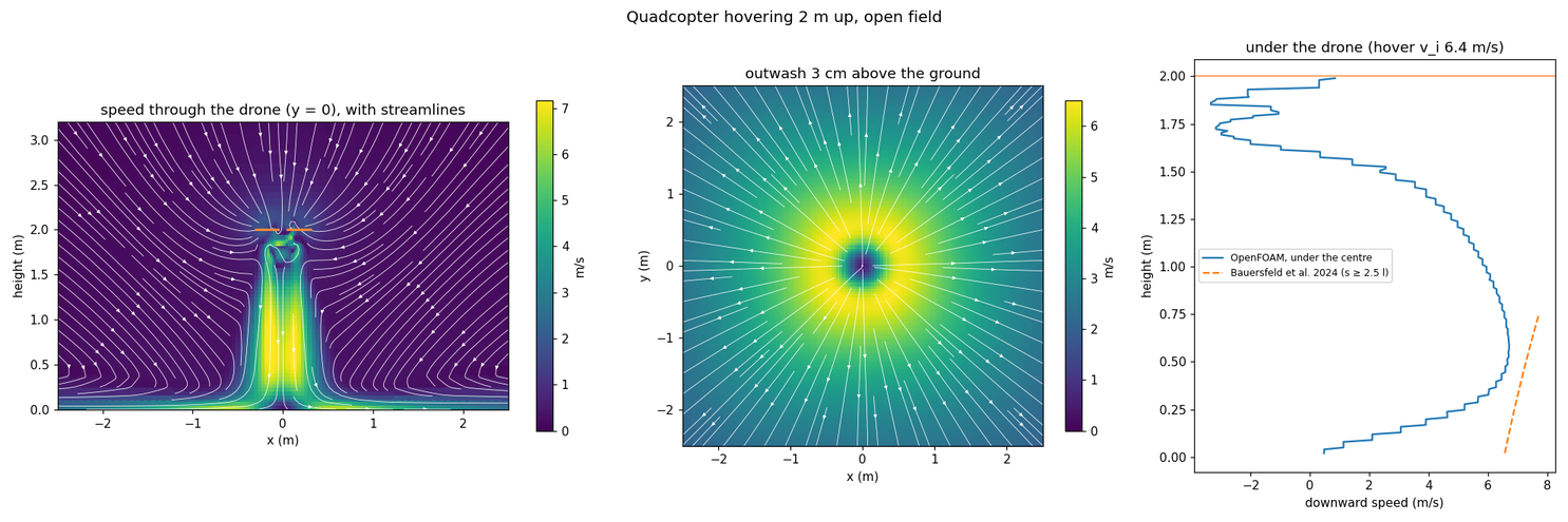
In the open, the jet under the drone peaks at 6.7 m/s about 0.5 m above the ground. Bauersfeld et al.’s fit gives 7.35 m/s there, about 10% more. Their measurements were also taken in the open, with no ground in the fit. Between the four rotor columns, just under the drone, the air rises: the known fountain of a multirotor.
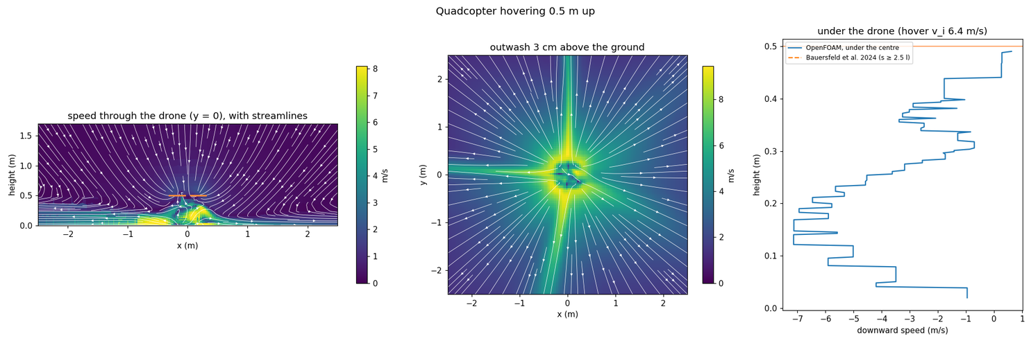
Low, at 0.5 m, the rotor jets reach the ground before they merge. Their wall jets meet along the arms in a cross and turn up under the drone at about 7 m/s. That lifts the frame (0.63 N) instead of pressing it down, and the outwash is half as strong again (9.5 m/s).
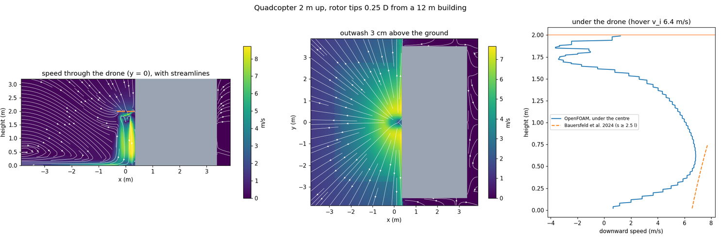
Beside a building, the wake hugs the wall, faster there (up to 8.7 m/s) than in the open. It spreads along the foot of the wall rather than round the drone. The rotors near the wall take more air through them and the far ones less (§2.7). The frame feels no side force (0.02 N), so the pull towards the wall comes through the rotors.
The live model covers the open-field jet within its references, the roof and wall-hugging wake (§2.6), the near-wall rotors (§2.7) and the fountain’s push on the frame (§2.8, fitted to the five heights above).
8. Live air: a lattice Boltzmann box¶
The fitted model (§2) is a set of rules, one per thing that has been measured. The alternative is
to compute the air itself every step, near the drone, as lagrange tunnel does offline. This
section measures whether that can run live, and how close it comes.
aerodynamics::LbmBox (modules/aerodynamics/lbm/src/LbmBox.cpp, GPU step
gpu/kernels/fields/lbm_box.slang) is a box of air round the drone:
D3Q19 lattice Boltzmann with the Smagorinsky eddy viscosity, as the tunnel (Krüger et al. 2017; Hou et al. 1996).
Each rotor is an actuator disc: its thrust pushes the air through Guo’s forcing (Guo, Zheng and Shi 2002) over a disc one cell thick. The cells’ weights are summed, so the air gets exactly the thrust.
The sides and top are open at ambient pressure. Flow leaving carries on; air drawn in comes by the pressure alone (carrying an inward speed in made the top of the box blow up). The bottom is a no-slip ground, or open.
The GPU stores the populations in half precision, less their rest weights (FP16S, Lehmann et al. 2022), two cells to a word. The step is bound by memory traffic, and this, with skipping the solid lookups in a box without solids, took the 5 cm box from 1.05× to 1.9× real time.
The CPU path is the reference (invariant 7);
test_lbm_boxchecks that the GPU agrees with it.
test_lbm_box also checks momentum theory (Leishman eq. 2.14): the downward momentum through a
plane 0.4 m under a lone disc carries its thrust within 2% (4.07 N of 4.00 N), and the speed at
the disc’s centre is 23% over the ideal induced velocity (the disc’s edge blurred over cells).
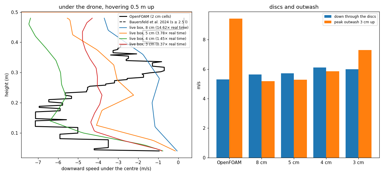
8.1 Speed and accuracy on an RTX 4060 Laptop GPU¶
tools/validation/lbm_hover.py CASE OUT runs lagrange_lbm_hover (installed with
lagrange_aerodynamics) with the rotors of a lagrange foam-hover case: a box 4 m × 4 m, from
the ground to 1 m over the drone, 3 s of air (2 s for the low case), the last second averaged.
Speeds are sampled the same way in both: over each disc’s plane, under the drone’s centre, and
3 cm over the ground. (The disc numbers here sample points on the disc plane, so OpenFOAM’s are
lower than §7’s cell averages.)
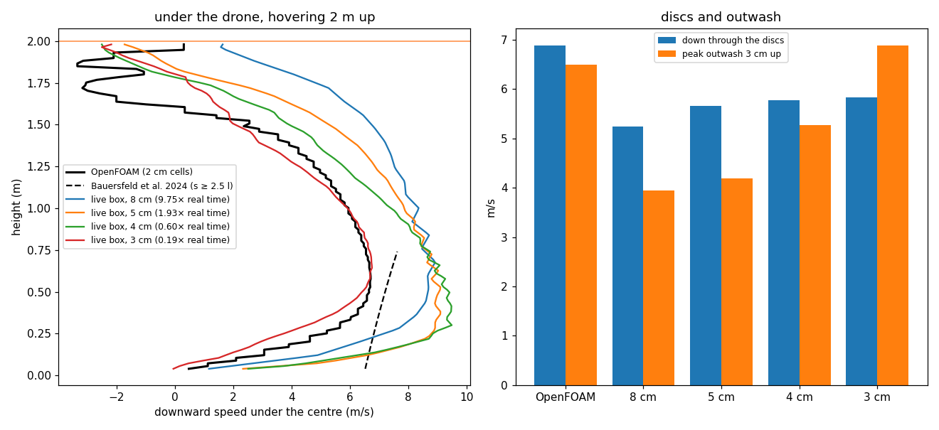
2 m up (OpenFOAM: discs 6.89 m/s, outwash 6.49 m/s):
Cells |
Cells in the box |
Real time |
Down through the discs |
Peak outwash |
Centreline against OpenFOAM |
Jet against Bauersfeld |
|---|---|---|---|---|---|---|
8 cm |
95k |
9.8× |
5.24 m/s |
3.94 m/s |
72% |
21% |
5 cm |
384k |
1.9× |
5.65 m/s |
4.20 m/s |
62% |
23% |
4 cm |
750k |
0.60× |
5.77 m/s |
5.27 m/s |
51% |
26% |
3 cm |
1.77M |
0.19× |
5.83 m/s |
6.89 m/s |
20% |
34% |
0.5 m up (OpenFOAM: discs 5.30 m/s, outwash 9.44 m/s, the fountain rising at up to 7.1 m/s under the centre):
Cells |
Real time |
Down through the discs |
Peak outwash |
Fountain under the centre |
|---|---|---|---|---|
8 cm |
14.6× |
5.63 m/s |
5.19 m/s |
up to 3.7 m/s, only near the drone |
5 cm |
3.8× |
5.72 m/s |
5.29 m/s |
up to 5.5 m/s |
4 cm |
1.45× |
6.12 m/s |
5.86 m/s |
up to 7.4 m/s |
3 cm |
0.37× |
5.99 m/s |
7.31 m/s |
up to 5.8 m/s |
The centreline error is the mean difference under the drone’s centre over the whole height, divided by OpenFOAM’s mean there. Most of it is the first half metre under the drone, where OpenFOAM’s frame (a solid there) makes the air rise between the rotors and the box has no frame. A 3 m box at 4 cm (427k cells) runs at 1.06× real time; at 3 cm (1M cells), 0.35×.
8.2 Go, at 4 cm¶
What it gets that the fitted model cannot. At 4 cm and finer, the box makes the fountain under a low drone (§6), rising at 5.8–7.4 m/s against OpenFOAM’s 7.1 m/s, and at 3 cm its outwash in the open is within 6% of OpenFOAM’s (4 cm: 19% under). Nothing in it is fitted to a drone, so it will also make interactions the rules don’t have: two drones’ wakes, a drone over a moving vehicle, wind round a building.
What it costs. On this laptop GPU, a 3 m box at 4 cm keeps up with real time. 3 cm, which matches OpenFOAM’s jet best (centreline within 20%), runs at a third of real time. 5 cm and coarser merge the four jets too early (outwash 35–40% low): too coarse to be worth it over the fitted model.
What it does not get. The air through the discs is 15–20% under OpenFOAM’s: a disc 3 cells across is blurred over its edge. In the low case the outwash is 22–38% under OpenFOAM’s 9.4 m/s, since a wall jet a few centimetres thick is one cell. Bauersfeld’s far jet is matched to 21–34%, no better than the fitted model, which was fitted to it.
So the box goes in as a choice (aerodynamics.downwash_model: lbm), with the cell size a setting
(4 cm by default) and the fitted model the default, the CPU fallback and Tier 0’s model. A finer
box runs slower than real time, and the scheduler’s real-time factor then drops; the run stays
correct. Grid refinement (fine cells only near the rotors) would be the next speed-up.
8.3 In a run: downwash_model: lbm¶
aerodynamics: { ..., downwash_model: lbm } (profiles/examples/quad_x500_live_air.yaml) puts the
run’s first multirotor in a box of live air (aerodynamics::LiveAir, owned by AeroDrag):
The box is 3 m across, from 2 m under the drone (down to the ground, with a floor, when the drone is within 2.5 m of it) to 1 m over it, in 4 cm cells (450k cells hovering 2 m up). It moves with the drone, on the grid of cells, once the drone has drifted 6 cells; the flow is carried over, and new cells start still. Scenery boxes (§2.6) are walls in it.
The rotors push it every 5 ms of air with their present thrust (
rotor/<j>/thrust,thrust_axis), as actuator discs.The wind (the mean wind at the drone) blows through it: where it blows in, it comes in, and new cells start in it, so the wake leans downwind in the flow itself (in
test_lbm_boxa disc’s jet half a metre down moves 0.43 m downwind in a 2 m/s crosswind). What the box gives back is the air’s departure from that wind, so the wind and the gusts are added once, as before; the gusts do not blow through the box.The air a rotor flies in (
rotor/<j>/air_velocity, whatbemrotors read) is the box’s air over its disc less the disc’s own: at the start the box runs a lone disc of the same radius in still air and measures what share of momentum theory’s induced velocity it makes, and that share of the rotor’s own induced velocity is taken off. What is left is everything else: the other rotors of the drone, the ground, walls. So the fitted wall effect (§2.7) is not added on top.Other robots in the box feel its air (drag on their links, their rotors’ air); outside it, and for every other multirotor, the fitted model (§2) stays, and dust still follows the fitted outwash (§2.5).
The viewer gets the box as
aero/air_box(Field3D, every second cell, 8 cm, rebuilt every 0.1 s), which the server samples foraero/wind_speedslices and the particles inside the box.Speed: the sample quadcopter hovering 2 m up runs at about 0.75× real time on the RTX 4060 Laptop GPU (the box’s steps take 1.1 s per second of air). The scheduler’s real-time factor drops; the run stays correct.
No hardware GPU (Tier 0, or only a software device): the fitted model runs, with a line on the console.
downwash_lbm_cpu: truein the module’s config runs the deterministic CPU reference instead (slow; the tests use it,DownwashPair.TheLiveAirBoxDrawsTheRotorsTogether). The GPU path is not bit-reproducible (invariant 7); the box is not in saved states, so a restored run starts it still.
Hovering 2 m up, each rotor of the sample flies in about 1.1 m/s of air drawn in towards the drone’s centre and 0.3–0.5 m/s more down than a lone rotor: OpenFOAM’s hover case (§7) had about 1.05 m/s inwards at each disc. The flow is unsteady, so the rotor speeds the controller needs move by about 1% (543–564 rad/s) where the fitted model holds them constant.
Live air: hovering, then down to half a metre
9. Against measured flight: NeuroBEM¶
Bauersfeld, Kaufmann, Foehn, Sun and Scaramuzza (“NeuroBEM: Hybrid Aerodynamic Quadrotor Model”,
RSS 2021) flew a 0.772 kg racing quadrotor (Armattan Chameleon 6” frame, 0.13 m arms, 5.1” three-
blade propellers) for 75 minutes in a Vicon hangar at up to 65 km/h and published the logs at
400 Hz: body velocity, angular rate, acceleration and the four measured motor speeds
(dataset; no licence stated, so it is downloaded, never
committed). From the measured motion the force and torque on the vehicle are m·a and
J·dω/dt + ω × Jω; lagrange_rotor_replay computes what Lagrange’s rotors make from the measured
motor speeds and motion, and tools/validation/neurobem.sh downloads the data, checks its SHA-256
and runs the authors’ 13 held-out test segments. Errors as their Table II gives them (RMS, N and
N·m; F and M over the three axes):
Model |
Fxy |
Fz |
Mxy |
Mz |
F |
M |
|---|---|---|---|---|---|---|
Their quadratic fit (Table II “Fit”) |
1.536 |
1.381 |
0.104 |
0.033 |
1.486 |
0.087 |
Their blade-element model (Table II “BEM”) |
0.803 |
1.265 |
0.090 |
0.017 |
0.982 |
0.074 |
Lagrange |
1.356 |
1.642 |
0.109 |
0.006 |
1.458 |
0.089 |
Lagrange |
1.142 |
2.088 |
0.115 |
0.009 |
1.524 |
0.094 |
Lagrange |
1.113 |
1.141 |
0.128 |
0.010 |
1.122 |
0.105 |
The propeller (assets/propellers/neurobem_5in_3blade_*.prop.yaml) has the radius, blade angle
(21.77° at the axis, −11° to the tip) and chord (17 to 7 mm) the authors measured; its sections
are our low-Reynolds-number NACA 6412, an assumption (theirs are not published, and their lift and
drag coefficients were identified for their own model, which has no tip loss). One parameter is
fitted, as they fitted theirs on a test stand.
The coefficient model is their quadratic fit: 1.46 N against 1.49 N.
bemcuts the force error by a quarter (1.12 N, 15 % of the weight), most of it in Fz as the vehicle climbs, descends and flies fast through its own inflow, and is best of all on yaw.It is 14 % behind their blade-element model on force, 41 % on Mxy. The difference is in the plane of the disc: they model blade flapping on a hinge spring identified from video of the spinning propeller (coning, and its forward and sideways tilt in edgewise flow); ours are rigid blades with a hub moment from the advancing blade’s lift (aerodynamics.md §2.1). Neither model has the frame’s drag or the rotors’ interference with each other.
Unfitted, the geometry alone gives 1.52 N: the 2° is the gap between a guessed section and the real one, about what a NACA chart’s zero-lift angle is uncertain by.
Owed: blade flapping (coning and tilt), the frame’s drag, a per-axis comparison of moments. The
arm geometry and spin directions are from their trajectory code (setupKingfisher.m) and the
logs; the rotors’ height above the centre of mass is taken as zero.